The main window of ModSim is the main entrance point to all modeling, simulation,
data visualization and import/export tasks.
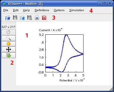
The central widget of the window (1)
describes a page that contains one or more data graphs (the figure shows an example
of a single graph that contains a cyclic voltammogram). A click with the left mouse button on a graph
activates it (background color changes from grey to white).
An activated graph can be modified both with the graphics toolbar
(2) and with the link
'Options->Graph Settings' (see below).
The toolbar (2) contains the following
actions (from top to bottom): 'rotate' (3D only), 'zoom', 'illuminate' (3D only),
'translate' and 'add data to' (2D only).
In order to perform a chosen graphics action you must keep the left mouse
button pressed and move the cursor in the desired direction
(for convenience, the zoom functionality is always provided by the right mouse
button).
To add data to an active graph, simply click on the 'add data to' icon.
Then, after the next simulation run, the output will appear as an additional
curve in the activated graph. In an analogous way, you can import data to
an activated graph (e.g. to compare experimental with simulated results).
Just activate a graph, click on the 'add data to' icon and import the data.
The file toolbar (3) offers a convient access to the 'File Menu' actions (see below). From left to right: 'open project', 'save project', 'import data to active graph', 'export data of active graph' (or 'export active graph as image'), 'print' and 'exit program'.
The Menu toolbar (4) provides the access to the menu items 'File', 'Edit', 'Help', 'Definitions', 'Options' and 'Simulation'. The specific actions are explained below.
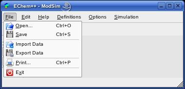
The settings of each ModSim dialog, as well as the current model
information can be saved in form of XML project files. The project
files can be loaded again into the program ('File->Open', 'File->Save').
Note that you should not modify the project files by hand (except if you
know what to do). A modified file may cause errors during anew 'File->Open'.
Import and export tasks can be performed by the 'File->Import Data', 'File->Export Data'
actions. Currently, only 2D data in ASCII text files can be imported (e.g. experimental
data recorded by the BAS100BW software). If the 'graphics toolbar->add data to' button is
pressed, the data are plotted as an additional curve within the active graph.
Otherwise a new graph is created in the page.
2D data can be exported as ASCII text files. However, active graphs (or the whole page,
if no graph is activated) can be exported in several file formats (EPS, PS, PDF, TEX).
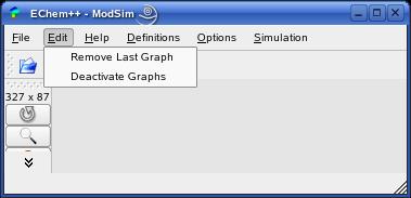
The 'Edit' menu provides two actions. 'Edit->Remove Last Graph' removes the last graph from the page (if any graph is shown). 'Edit->Deactivate Graphs' deactivates an active graph. Note that only a single graph can be active. Each time you click on a non-active graph, it gets activated. Simultaneously, the former active graph gets deactivated.
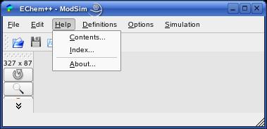
The 'Help' menu provides three actions. 'Help->Contents' opens the HTML help browser of ModSim. You will find this user manual there, but also the complete C++ class reference and documentation of the EChem++ libraries. 'Help->About' opens some licence information of the current ModSim release
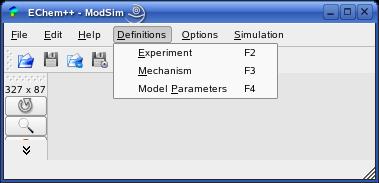
The 'Definitions' menu contains the three actions of ModSim's modeling pipeline.
'Definitions->Experiment' (shortcut F2) opens the Experiment Dialog
(see below). There you can define the geometry
and transport model, as well as the excitation functions. After a proper
definition, the 'Mechanism' action will be enabled.
'Definitions->Mechanism' (shortcut F3) opens the Mechanism
Dialog, a graphical front-end to the Ecco compiler (see below).
There, the electrochemical reaction mechanism, as well as non-standard model kinetics
(if desired) can be defined. After an error-free compilation, the next action 'Model Parameters'
will be enabled.
'Definitions->Model Parameters' (shortcut F4) opens the
Model Parameters Dialog
(see below). There, you can specifiy all relevant model
parameters according to the compiled reaction mechanism. After that, the program is
ready for simulation.
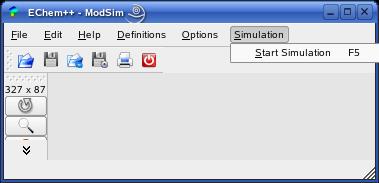
In order to run a simulation, simply press the F5 key, or click on the 'Simulation->Start Simulation' action. Note that the action is only enabled, if all model settings have been done without failure.
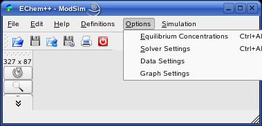
The 'Options' menu contains four actions that open the according option dialogs.
See the dialogs for details:
| Action | Dialog |
| 'Options->Equilibrium Concentrations' | Initial Equilibrium Concentrations |
| 'Options->Solver Settings' | Solver Settings |
| 'Options->Data Settings' | Data Storage & Visualization |
| 'Options->Graph Settings' | Graph Settings |
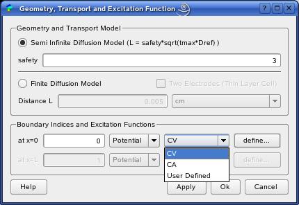
The ExperimentDialog enables the definition of the currently supported
geometry and transport models, as well as excitation functions.
In the button group 'Geometry and Transport Model'
you can choose one of the supported models:
| 'Semi Infinite Diffusion' | Linear diffusion field to a single planar working electrode. The geometry is represented by a 1D interval, [0,L]. The electrode surface is located at x=0. The diffusion layer limit is x=L. The thickness L of the diffusion layer is approximated by a safety factor 'safety' multiplied by the Nernst diffusion layer model sqrt(tmax*Dref), where tmax is the total experiment duration and Dref the reference diffusion coefficient (usually taken as the maximum of all diffusion coefficients). |
| 'Finite Diffusion' | Linear diffusion field between an electrode and an inert wall or
between two opposed planar working electrodes (thin layer cell). The geometry is represented by a 1D interval, [0,L]. One electrode surface is located at x=0. The other inert wall or electrode is located at x=L. The 'Distance L' of the thin layer can be defined. |
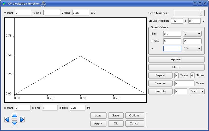
The Figure shows the dialog for the creation of a cyclic voltammetric
excitation function. Such dialogs describe the graphical front-ends to
various classes from the excitation function template library[2].
In principle, electrochemical excitation functions are composed of several
segments that describe the functional relationship between time
and potential (or current for current-controlled experiments).
Thus, in the example above, the function is composed by two linear
E-t-segments (scans). The easiest way to gradually create the
excitation function is to specify the values that defines a segment
(here called 'Scan Values' on the right)
and press the 'Append'-Button.
In our example, the first segment starts at a initial potential
of Einit = 0 V and reaches a value of Emax = 0.5 V with a scan
rate of v = 1 V/s.
By pressing the 'Append'-Button the segment
is created, pushed into the excitation function and, finally, drawn as black
line within the graph on the left side of the dialog.
The following segments can be either defined as before (specify the
new values and press 'Append') or by pressing the
'Mirror'-Button. It is important to note, that
a mirrored segment (firstly drawn as blue line) has to be accepted
by the 'Append'-Button (the blue line becomes
black).
Other functionalities of the dialog are less important and will be
described in later versions of this manual.
In order to accept yout settings, press
'Ok'.
Now, the excitation function is stored at the respective boundary
surface within the geometry for simulation.
Reaction Mechanism [Up]
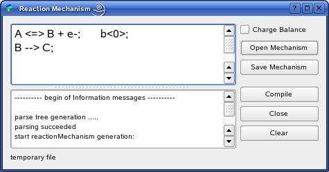
The MechanismDialog is the graphical front-end of the Ecco compiler
described in [1].
Here, you can specify the electrochemical and chemical reaction
model. The figure shows the example of a heterogeneus one-electron
oxidation
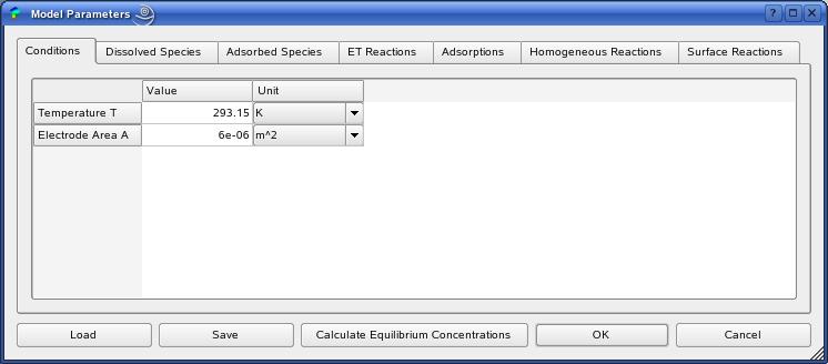
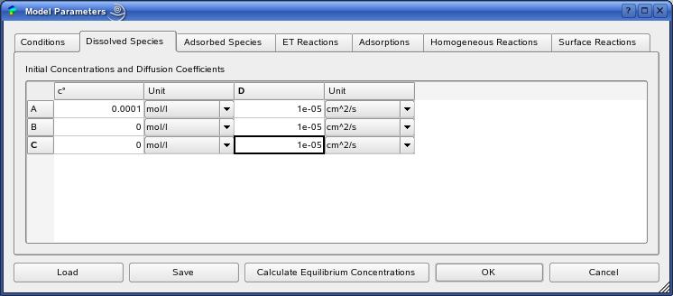
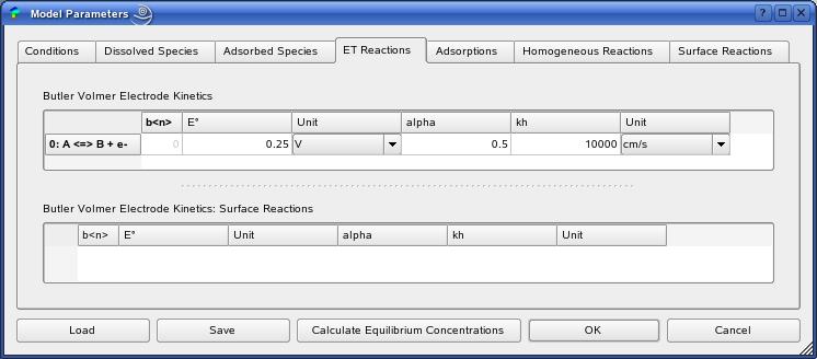
The definition of all model parameters follows within the ModelParamtersDialog.
The button 'Calculate Equilibrium Concentrations' starts
the calculation of the initial equilbrium state of the reaction mechanism.
The concentration values in the species tabs 'Dissolved Species'
and 'Adsorbed Species' will be replaced by the
result of this caclulation. Usually, the program shows a short message if the
equilbrium is reached. Depending on the settings within the EquilibriumDialog
(see below) the simulated concentration profiles are
shown within the main window after calculation.
!!Note: After a successfull equilbrium calculation the simulation of the electrochemical
model can be started (see above).
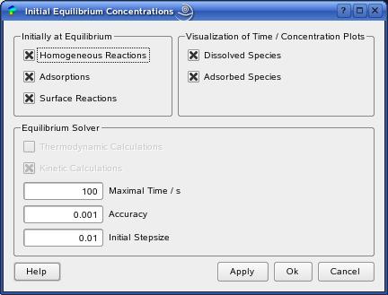
The EquilibriumDialog provides all settings concerning the calculation of the initial values for the electrochemical simulation model, i.e. the concentration distribution of all species in the electrochemical cell at the moment in which every reaction has reached its equilibrium state.
Per default, we assume that all homogeneous reactions, adsorptions and surface reactions have reached their equilibrium state at the beginning of the electrochemical experiment. In order to change this assumption, you can switch off the reaction checkboxes in the button group 'Initially at Equilibrium'.
For the calculation of the equilibrium state, we numerically
solve a system of ordinary differential equations (ODE system)
that describe the concentration field of each species
(currently only this "kinetic calculation" is fully supported).
The ODE system is created based on the output of
the Ecco compiler.
The equilibrium is reached as soon as all possible mass
action laws of the reactions are fulfilled.
The numerical solver demands for three parameters that
can be defined within the group 'Equilibrium Solver'.
These are the 'Maximal Time' in seconds
that determines the maximal time the integration steps
are performed. Note that this is not a real time value - usually the numerical
solver is much faster.
The solver stops as soon as the equilibrium is reached.
As noted before, the stopping criterion is complied, if
all laws of mass actions are fulfilled.
Therefore, we observe the residual function R = K - MAL(c),
where K is the equilibrium constant of a reaction and
MAL(c) is the accoring mass action law.
If R becomes lower than the 'Accuracy'
value, the solver stops and the equilibrium state is reached.
The last value, 'Initial Stepsize', is
the inital time step size of the numerical solver.
The solver is an implementation of the Shampine Rosenbrock integrator
described in the book [4].
The ouput of the equilibrium calculation describes
time-concentration curves that are plotted within the
main window. The last concentration points of these
curves are the initial values for the subsequent
electrochemical simulations.
In the button group 'Visualization
of Time / Concentration Plots', you can
switch off the visualization of the concentration plots.
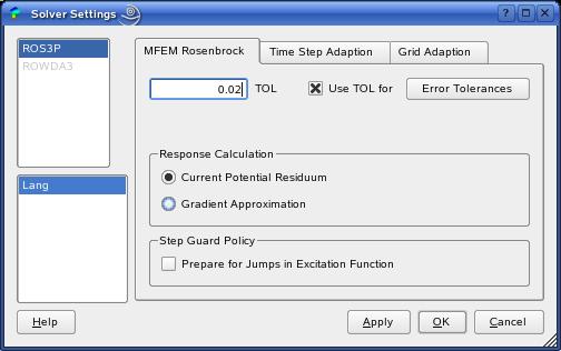
The SolverDialog provides all settings of the adaptive finite
element algorithm that solves the electrochemical reaction-diffusion
equations. For example, the overall relative error tolerance can be
specified in the 'TOL' field (a value of
0.02 means 2%). Then, the estimated errors within the curves are kept
below that treshold.
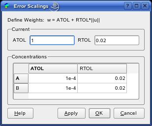
The solution process also depends on the values specified as absolute
error tolerances (ATOL-values on the right). Low ATOL-values are recommended.
The algorithms work well for relative error tolerances between 5% and 0.1%
and low ATOL-values. If you observe bad/distorted results, you might
decrease these values carefully.
The current response can be calculated by two different solution concepts ('Response Calculation', left Figure).
The strategy based on the 'Current Potential Residuum' solves a differential-algebraic
equation system at the electrode surfaces and enables the error control also
within the electrochemical response (this is the default setting).
The 'Gradient Approximation' strategy calculates the current in a post-processing
step from the concentration profiles.
Moreover, for unsteady excitation functions, you must enable the 'Step Guard Policy'.
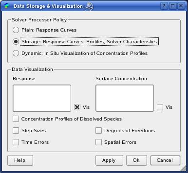
Data storage and visualization settings are managed by the DataDialog.
In the button group Solver Processor Policy,
you can choose three behaviour types of the numerical algortihm.
The 'Plain' processor policy only stores
the response curve(s), i.e. the current-potential or current-time
curves for potential-controlled experiments. That might be the most
efficient configuration, since some function calls during simulation
are avoided. However, in order to store and plot concentration
profiles and solver characteristics (step size, error and grid evolutions)
you must choose the 'Storage' policy.
The 'Dynamic' configuration shows the
concentration profiles evolution during simulation in real time.
In the lower button group 'Data Visualization'
the plots of the specific data can be switched on and
off by the corresponding check boxes.
For the visualization of the 'Concentration Profiles of Dissolved
Species', an extra plot window will be opened (see below).
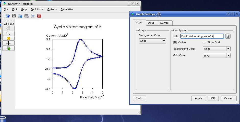
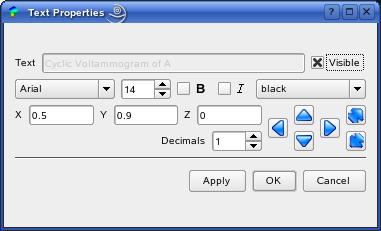
The settings for active graphs can be changed by clicking (left mouse button) on the desired graph and choose 'Options->Graph Settings' in the menu (see above). The GraphDialog contains three tabs: 'Graph', 'Axes' and 'Curves' that provide all available changes for the visualization. In the 'Graph' tab you can change the look for the whole graph and the axis system. By pressing the small text icon beside the title line edit, you can change the position of the text, as well as general font settings in the TextPropertiesDialog:
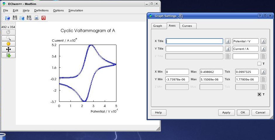
The look of all axes can be configured in the 'Axes' tab ...
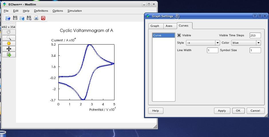
... and all settings concering the plotted curves can be changed in the 'Curves' tab. You will see all changes within the main window by pressing the 'Apply' button.
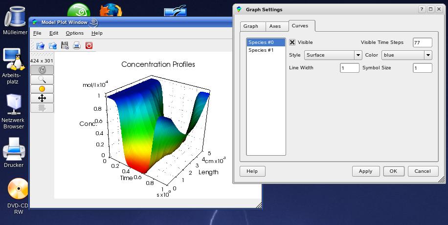
The concentration evolution within the electrochemical cell
can be visualized by a 3D plot. Therefore, you must
activate the 'Storage' policy before
simulation and switch on the 'Concentration Profiles of
Dissolved Species' check box in the DataDialog.
With 'Options->Graph Settings' in the Model Plot
Window you can access the GraphDialog in order to modify the look of the plot.
The data are shown with a rather low time resolution ('Visible
Time Steps'). You can increase this value until a certain maximum value.
| Quantity | quantity.sourceforge.net |
| Spirit | spirit.sourceforge.net |
| GiNaC | www.ginac.de |
| GMM++ | www-gmm.insa-toulouse.fr/getfem/gmm_intro |
| VTK | public.kitware.com/VTK |
| Qt | www.trolltech.com |
| tree.hh | www.aei.mpg.de/~peekas/tree/ |
| TinyXml | www.grinninglizard.com/tinyxml/ |